Dynamic Product Pricing Using Python
by
Pritish Jadhav - Sun, 03 Jan 2021
Dynamic Price Optimization - Single Product
- The year 2020 was arguably one of the most difficult years on the professional as well as personal fronts. The COVID-19 pandemic hit us hard and forced us to seek safe havens by practically giving up on socializing.
- The pandemic also severely affected business and economic growth across industries and nations.
- It also changed the way we have been conducting businesses until now. The lockdown and physical distancing measures presented a unique challenge to the brick and mortar retail stores that rely heavily on foot traffic for moving their products.
- The pandemic has forced people to adopt online shopping more comprehensively for their daily needs.
- The whole shift in paradigm has prompted businesses to start building an online presence to sustain, survive, and eventually grow in the post-pandemic world.
- However, selling online is not new and trivial. Brands have been selling online for quite some time and the competition in certain categories is often cut-throat.
- Product pricing plays a pivotal role at various stages of a product lifecycle and has a direct impact on a brand's bottom line.
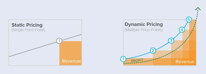
- In this blog post, we shall use the explore-exploit strategy for determining the optimal price for a SINGLE product.
In [6]:
import numpy as np
import pandas as pd
import random
import matplotlib.pyplot as plt
from typing import NamedTuple, List
from mypy_extensions import TypedDict
from collections import defaultdict
import ipywidgets as widgets
import scipy.stats as stats
from ipywidgets import interact, interactive, fixed, interact_manual

from IPython.display import HTML
display(HTML('<style>.prompt{width: 0px; min-width: 0px; visibility: collapse}</style>'))
display(HTML("<style>.container { width:100% !important; }</style>"))
A true demand model (Unobserved in Real Life) -
- To kick things off, lets define a mathematical model for determining the "true" demand for the product under consideration.
- It is important to note that this true demand is unobserved in a real-life scenario.
- We will use this model to generate observed values that will be used by the algorithm for updating the beliefs.
- We shall use a simple linear model with a slope and intercept to define the true demand.
${\theta_1}$ -> intercept
${\theta_2}$ -> slope
Things in the wild are hardly linear but hopefully, this will lay the foundation for the problem that we are trying to solve.
For the sake of this blog post, we shall choose ${\theta_1} = 50$ and ${\theta_2} = -7$. Please note that these values have been chosen heuristically.
In [ ]:
theta_1 = 50
theta_2 = -7

plot_prices = np.linspace(1.99, 4.99, 400)

# Visualize the true demand model

true_demand = theta_1 + (theta_2 * plot_prices)

plt.figure(figsize = (5,5))
plt.plot(plot_prices, true_demand, label = "true demand")
plt.plot(plot_prices, plot_prices * true_demand, label = "revenue")
plt.axvline(x = 3.56, linestyle='--',color = 'r')

plt.plot(3.56, 25.017, '--bo', color = 'red')
# plt.annotate((3.56, 25.017), [3.56, 25.017])

plt.plot(3.56, 89.28, '--bo', color = 'red')
plt.annotate((3.56, 89.28), xy = [3.56, 89.28],
             xytext=(30, -50),
             textcoords = "offset points",
             arrowprops=dict(arrowstyle="->", color='red'))
plt.annotate((3.56, 25.017), xy = [3.56, 25.017],
             xytext=(30, 50),
             textcoords = "offset points",
             arrowprops=dict(arrowstyle="->", color='red'))

plt.legend()
In [ ]:
print(true_demand[np.argmax(true_demand * plot_prices)])
print(plot_prices[np.argmax(true_demand * plot_prices)])

np.max(true_demand * plot_prices)
A Note on the true optimal price -
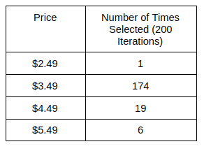
- To keep things real, we shall be testing a finite set of prices for our product under consideration.
- The prices to be tested are \$2.99, \\$3.99, \$4.99, \\$5.99.
- It can be seen from the above graph that the price of \$3.99 is the most optimal with a demand of 50 - 7*3.99 = 22.07 and revenue of \\$88.05.
- So at the end of this blog, our algorthm should be able to explore all prices but exploit the price of \$3.99 i.e select \\$3.99 more often as compared to other price points.
Algorithm Walkthrough -
In this section, let's discuss a few approaches and finalize the algorithm that we would adopt for solving the problem -
The Greedy approach -
- A naive and greedy way of determining the optimal price of a product would be to collect the historical data and choose the price that maximizes revenue.
- However, this approach is suboptimal because it prevents us from choosing prices that do not have enough data. As a result, we will never know if the selected price is indeed the most optimal.
- Hence the greedy algorithm is designed for maximizing the short-term gains while missing out on exploring all viable options.
The $\epsilon$ Greedy Algorithm -
- The $\epsilon$ greedy algorithm alleviates the critical drawback of the greedy algorithm by adopting the greedy approach with probability $1- \epsilon$ and explores with a probability $\epsilon$.
- Typically, the value of $\epsilon$ is chosen to be small.
- In the exploration phase, the algortihm would allocate experimental actions using a uniform distribution. Therefore, it would choose each experimental action an equal number of times.
- As a result,the $\epsilon$-greedy algorithm fails to discount actions with a very low probability of being optimal.
Thompson Sampling to the rescue -
- The Thompson sampling approach solves the drawbacks from earlier mentioned approaches where we kick off the process by attaching prior beliefs to each of the available options.
- At every time step, we select the optimal option, observe and update the belief.
- For determining the optimal price for a product using Thompson sampling, we would assume the demand to be a Poisson process with its parameter $\lambda$ being gamma distributed with parameters $\alpha$ and $\beta$.
- Then, the pseudocode for Thompson sampling in the context of Dynamic Pricing for a single product would be -
Psuedocode -
Define a prior distribution $p(\lambda) \sim gamma(\alpha, \beta)$ for each of the price points to be tested.
At each time step t-
- sample demands for each price points i.e d $\sim$ p($\lambda)$
- Find the optimal price -
$price^*$ = $argmax_{price}$ [price * demand] - Offer the optimal price and observe the true demand ($d_t$).
- Update the belief for the selected price point using -
$\beta = \beta +1 $
In [ ]:
# define the prices to be tested
prices_to_test = np.arange(2.49, 5.99, 1)
# define the prior values for the alpha and beta that define a gamma distribution
alpha_0 = 30.00
beta_0 = 1.00
def sample_true_demand(price: float) -> float:
"""
np.poisson.random -> https://numpy.org/doc/stable/reference/random/generated/numpy.random.poisson.html
"""
demand = theta_1 + theta_2 * price
return np.random.poisson(demand, 1)[0]
class priceParams(TypedDict):
price: float
alpha: float
beta: float
p_lambdas = []
for price in prices_to_test:
p_lambdas.append(
priceParams(
price=price,
alpha=alpha_0,
beta=beta_0
)
)
class OptimalPriceResult(NamedTuple):
price: float
price_index: int
def get_optimal_price(prices: List[float], demands: List[float]) -> OptimalPriceResult:
index = np.argmax(prices * demands)
return OptimalPriceResult(price_index = index, price = prices[index])
def sample_demands_from_model(p_lambdas: List[priceParams]) -> List[float]:
return list(map(lambda v: np.random.gamma(v['alpha'], 1/v['beta']), p_lambdas))
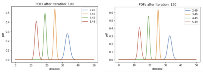
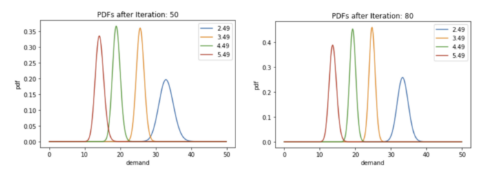
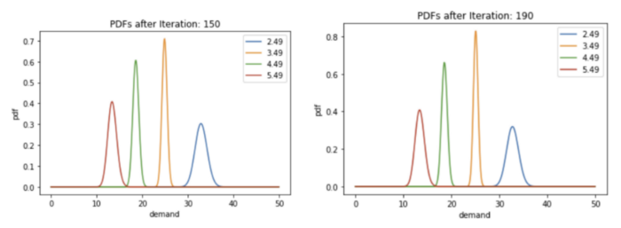
def plot_distributions(gamma_distributions: List[priceParams], iteration: int):
x = np.arange(0, 50, 0.10)
for dist in p_lambdas:
y = stats.gamma.pdf(x, a=dist["alpha"], scale= 1/dist["beta"])
plt.plot(x, y, label = dist["price"])
plt.xlabel("demand")
plt.ylabel("pdf")
plt.title(f"PDFs after Iteration: {iteration}")
plt.legend(loc="upper right")
plt.show()
In [ ]:
# Thompson sampling for solving the explore-exploit dilema.


price_counts = defaultdict(lambda: 0)

for t in range(200):
    demands = sample_demands_from_model(p_lambdas)

    optimal_price_res = get_optimal_price(prices_to_test, demands)

    # increase the count for the price
    price_counts[optimal_price_res.price] += 1

    # offer the selected price and observe demand
    demand_t = sample_true_demand(optimal_price_res.price)

    # update model parameters
    v = p_lambdas[optimal_price_res.price_index]
    v['alpha'] += demand_t
    v['beta'] += 1

    if t%10 == 0:
        plot_distributions(p_lambdas, t)

Next Steps -
- The concepts discussed in this blog post lays the foundation for building more complex demand distribution models instead of sticking to linear relationships.
- It is worth exploring different techniques including MCMC simulations for building and simulating complex distributions.
- The above formulation works for a single product but in real-world applications, we would want to experiment for multiple products along with a bunch of constraints.