The Curious Case of Convex Functions

The Curious Case of Convex Functions¶

• Most of the introductory courses for Machine Learning cover algorithms like Linear Regression and Logistic Regression with varying degrees of detail.
• The resources are plentiful for grasping the nitty gitties involved. However, I rarely found traditional courses diving into proving the convexity of MSE loss function.
• Most of the online resources often skim through the part where they define the cost function for Regression Algorithms using MSE where the cost function is claimed to be a convex function.
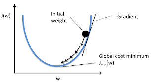
• The convexity property unlocks a crucial advantage where the local minima of a convex function is also a global minima.
• This ensures that a model can be trained where the loss function is minimized to its globally minimum value.

Proving Convexity -¶

• In this blog post, we shall work through the concepts needed to prove the convexity of a function.
• So hang in tight and by the end of this article, you would have a better understanding of -

a. Symmetric Matrices.
b. Hessian Matrices.
c. Positive and Negative Definite/Semidefinite Matrices.
d. Proving convexity of functions.

Without much further ado, let's jump into it.

Basics of Matrices -¶

We shall touch base on some of the basic concepts in Matrices that will help us in proving the convexity of a function. These basics are typically covered in Undergraduate Courses and should sound familiar to you.

1. Square Matrix -

Given a matrix X of dimensions $m \times n$, X is a square matrix iff (if and only if) m = n. In other words, A matrix 'X' is called a square matrix if the number of matrix rows is equal to the number of columns.

$$ \begin{align} X = \begin{bmatrix} 1 & 2 & 3 \\ 4 & 5 & 6 \\ 8 & 9 & 10 \end{bmatrix}_{3 \times 3} \end{align} $$

In the above example, since the number of rows (m) = number of columns (n), X can be termed as a square matrix.

2. Symmetric Matrix -¶

A square matrix 'X' is termed as symmetric if $x_{ij} = x_{ji}$ for all i and j where i, j denotes the ith row and jth column respectively. In other words, X is symmetric if the transpose of X is equal to matrix X.

i.e, $$ \begin{align} X^T = X \end{align} $$

3. Hermitian Matrix -¶

A square matrix X is self-adjoint or a Hermitian matrix if -

$$ \begin{align} \overline{X^{T}} = X = X^{H} \end{align} $$

Note that the terms self-adjoint and Hermitian can be used interchangeably.

4. Hessian Matrix -¶

The Hessian of a multivariate function $f(x_1, x_2, ...x_n)$ is a way for organizing second-order partial derivatives in the form of a matrix.

Consider a multivariate function $ f(x_1, x_2, ...x_n) $ then its Hessian can be defined as follows -

$$ \begin{align} H_f = \begin{bmatrix} \frac{\partial ^2 f}{\partial x_1^2} & \frac{\partial^2 f}{\partial x_1 \partial x_2} & \cdots & \frac{\partial ^2 f}{\partial x_1 \partial x_n} \\ \frac{\partial ^2 f}{\partial x_2 \partial x_1} & \frac{\partial^2 f}{\partial {x_2}^2 } & \cdots & \frac{\partial^2 f}{\partial x_2 \partial x_n} \\ \vdots & \ddots & \cdots & \vdots\\ \frac{\partial ^2 f}{\partial x_n \partial x_1} & \frac{\partial^2 f}{\partial x_n \partial x_2 } & \cdots & \frac{\partial^2 f}{\partial {x_n}^2 } \\ \end{bmatrix} \end{align} $$

Note that a Hessian matrix by definition is a Square and Symmetric matrix.

5. Positive Definite and Semidefinite Matrices -¶

You may have seen references about these matrices at multiple places but the definition and ways to prove definitiveness remains elusive to many. Let us start with the text definition -

\begin{align} A \; n \times n \; square \; matrix \; X \; is \; Positive \; Definite \; if \;\;\; a^TXa \; > \; 0 \; \forall a \; \in \; \mathbb R^n. \end{align}

Similarly,

\begin{align} A \; n \times n \; square \; matrix \; X \; is \; Positive \; Semidefinite \; if \;\; a^TXa \geq 0 \; \forall \; a \in \; \mathbb R^n. \end{align}

The same logic can be easily extended to Negative Definite and Negative Semidefinite matrices.

\begin{align} A \; n \times n \; square \; matrix \; X \; is \; Negative \; Definite \; if \;\; a^TXa \; < \; 0 \; \forall a \; \in \; \mathbb R^n. \end{align}

And finally,

\begin{align} A \; n \times n \; square \; matrix \; X \; is \; Negative \; Semidefinite \; if \;\; a^TXa \leq 0 \; \forall \; a \in \; \mathbb R^n. \end{align}

• However, while checking for Matrix Definiteness, manually validating the condition of every value of x is not an option.
• So let us try and break this down even further.

Eigen Values and Eigen Vector -¶

We know that an eigenvector is a vector whose direction remains unchanged when a linear transformation is applied to it.

Mathematically,

$$ \begin{align} Xa = \lambda a \tag{1} \end{align} $$

Where, $\lambda $ represents a scalar called the eigenvalue. This simply means that the linear transformation X on a can be completely defined by $\lambda $.

pre-multiplying eq.(1) by $a^T$ gives -

$$ \begin{align} a^TXa = a^T \lambda a \tag{2} \end{align} $$

since $\lambda $ in eq.(2) is a scalar we can write eq.(2) as - $$ \begin{align} a^TXa = \lambda a^T a = \lambda <a, a> \tag{3} \end{align} $$ where,
$<x, y>$ represent the dot product, $x^Ty$

Analysis¶

• It is easy to see that the dot product of a with $a^T$ will always be positive.
• Referring back to the definition of positive definite matrix and eq(3), $a^TXa$ can be greater than zero if and only if $\lambda$ is greater than zero.

Derived Definition for Matrix Definiteness -¶

Based on pointers mentioned in above Analysis we can tweak the formal definitions of Matrix Definiteness as follows -

1. A Symmetric Matrix 'X' is Positive Definite if $\lambda_{i} > \; 0 \;\; \forall i$
2. A Symmetric Matrix 'X' is Positive Semi-Definite if $\lambda_{i} \geq \; 0 \;\; \forall i$
3. A Symmetric Matrix 'X' is Negative Definite if $\lambda_{i} < \; 0 \;\; \forall i$
4. A Symmetric Matrix 'X' is Negative Semi-Definite if $\lambda_{i} \leq \; 0 \;\; \forall i$

Alternate Definition for Determining Matrix Definiteness -

1. Computing Eigenvalues for large matrices often involves solving linear equations.
2. Large Matrices involve solving linear equations in a large number of variables.
3. Hence, It may not always be feasible to solve for Eigen Values.

An Alternate Theorem for Determining Definiteness of Matrices comes to the rescue -

Theorem -¶

1. A Symmetric Matrix 'X' is Positive Definite if $D_k > \; 0 \;\; \forall k$ Where $D_k$ represents the kth Leading Principal Minor.
2. A Symmetric Matrix 'X' is Positive Semi-Definite if $\bigtriangleup_k \geq \; 0 \;\; \forall k$ Where $\bigtriangleup_k$ represents the kth Principal Minor.
3. A Symmetric Matrix 'X' is Negative Definite if $D_k < \; 0 \;\; \forall k$ Where $D_k$ represents the kth Leading Principal Minor.
4. A Symmetric Matrix 'X' is Negative Semi-Definite if $\bigtriangleup_k \leq \; 0 \;\; \forall k$ Where $\bigtriangleup_k$ represents the kth Principal Minor.

Principal Minors of a Matrix -¶

• For a Square Matrix X, a Principal Submatrix of order k is obtained by deleting any (n-k) rows and corresponding (n-k) columns.
• The determinant of such a Principal Submatrix is called the Principal Minor of matrix X.

Leading Principal Minors of a Matrix -¶

• For a Square Matrix X, a Leading Principal Submatrix of order k is obtained by deleting last (n-k) rows and corresponding (n-k) columns.
• The determinant of such a Leading Pricipal Submatrix is called as the Leading Principal Minor of matrix X.

Proving / Checking Convexity of a function -¶

With all the relevant definitions and theorem covered in previous sections, we are now ready to define checks for determining the convexity of functions.

A function f(x) defined over n variables on an open convex set $S$ can be tested for convexity using following criteria -

If $X^H$ is the Hessian Matrix of f(x) then -

• f(x) is strictly convex in $S$ if $X^H$ is a Positive Definite Matrix.
• f(x) is convex in $S$ if $X^H$ is a Positive Semi-Definite Matrix.
• f(x) is strictly concave in $S$ if $X^H$ is a Negative Definite Matrix.
• f(x) is concave in $S$ if $X^H$ is a Negative Semi-Definite Matrix.

Example -¶

Consider an equation of Quadratic form -

$$ \begin{align} f(x_1, x_2, x_3) = 5x_1^2 - 2x_1x_2 + 2x_2^2 + x_3x_2 + x_3^2 \end{align} $$

STEP 1 - Computing the Hessian¶

The Hessian of $f(x_1, x_2, x_3)$ can be defined as follows - $$ \begin{align} X^H = \begin{bmatrix} \frac{\partial{f^2}}{\partial{x_1^2}} & \frac{\partial{f^2}}{\partial{x_1x_2}} & \frac{\partial{f^2}}{\partial{x_1x_3}} \\ \frac{\partial{f^2}}{\partial{x_2x_1}} & \frac{\partial{f^2}}{\partial{x_2^2}} & \frac{\partial{f^2}}{\partial{x_2x_3}} \\ \frac{\partial{f^2}}{\partial{x_3x_1}} & \frac{\partial{f^2}}{\partial{x_3x_2}} & \frac{\partial{f^2}}{\partial{x_3^2}} \\ \end{bmatrix} \end{align} $$

\begin{align} \\ \frac{\partial{f^2}}{\partial{x_1^2}} & = \frac{\partial{}}{\partial{x_1^2}}(5x_1^2 - 2x_1x_2 + 2x_2^2 + x_3x_2 + x_3^2) \\ & = \frac{\partial{}}{\partial{x_1}}(10x_1 -2x_2) \\ & = 10 \end{align}

Similarly,

\begin{align} \\ \frac{\partial{f^2}}{\partial{x_1x_2}} & = \frac{\partial{}}{\partial{x_1x_2}}(5x_1^2 - 2x_1x_2 + 2x_2^2 + x_3x_2 + x_3^2) \\ & = \frac{\partial{}}{\partial{x_1}}(-2x1 + 4x_2 + 1) \\ & = -2 \\ & = \frac{\partial{f^2}}{\partial{x_2x_1}} \end{align}\begin{align} \\ \frac{\partial{f^2}}{\partial{x_1x_3}} & = \frac{\partial{}}{\partial{x_1x_3}}(5x_1^2 - 2x_1x_2 + 2x_2^2 + x_3x_2 + x_3^2) \\ & = \frac{\partial{}}{\partial{x_1}}(1x_2 + 2x_3) \\ & = 0 \\ & = \frac{\partial{f^2}}{\partial{x_3x_1}} \end{align}\begin{align} \\ \frac{\partial{f^2}}{\partial{x_2^2}} & = \frac{\partial{}}{\partial{x_2^2}}(5x_1^2 - 2x_1x_2 + 2x_2^2 + x_3x_2 + x_3^2) \\ & = \frac{\partial{}}{\partial{x_2}}(-2x_1 + 4x_2 + x_3) \\ & = 4 \end{align}\begin{align} \\ \frac{\partial{f^2}}{\partial{x_2x_3}} & = \frac{\partial{}}{\partial{x_2x_3}}(5x_1^2 - 2x_1x_2 + 2x_2^2 + x_3x_2 + x_3^2) \\ & = \frac{\partial{}}{\partial{x2}}(x_2 + 2x_3) \\ & = 1 \\ & = \frac{\partial{f^2}}{\partial{x_3x_2}} \end{align}\begin{align} \\ \frac{\partial{f^2}}{\partial{x_3^2}} & = \frac{\partial{}}{\partial{x_3^2}}(5x_1^2 - 2x_1x_2 + 2x_2^2 + x_3x_2 + x_3^2) \\ & = \frac{\partial{}}{\partial{x_3}}(x_2 + 2x_3) \\ & = 2 \end{align}$$ \begin{align} X^H = \begin{bmatrix}10 & -2 & 0 \\ -2 & 4 & 1 \\ 0 & 1 & 2\end{bmatrix} \end{align} $$

Step 2 - Compute Leading Principal Minors -¶

for k = 3, delete last (3-3) =0 rows and (3-3) = 0 columns $$ \begin{align} \\ D_{k} & = D_{3} \\ &= \begin{vmatrix}10 & -2 & 0 \\ -2 & 4 & 1 \\ 0 & 1 & 2 \\ \end{vmatrix} \\ & = 62 \end{align} $$

for k = 2, delete last (3-2) =1 rows and corresponding (3-2) = 1 columns $$ \begin{align} \\ D_{k} & = D_{2} \\ &= \begin{vmatrix}10 & -2 \\ -2 & 4 \\ \end{vmatrix} \\ & = 36 \end{align} $$

for k = 1, delete last (3-1) =2 rows and corresponding (3-1) = 2 columns $$ \begin{align} \\ D_{k} & = D_{1} \\ & = D_1 \\ &= \begin{vmatrix}10 \\ \end{vmatrix} \\ & = 10 \end{align} $$

Since $D_1 > 0 $, $D_2 >0 $ and $D_3 > 0$, Hessian of $f(x_1, x_2, x_3)$ is Positive Definite.

Step 3 - Comment on Convexity -¶

• Since Hessian of $f(x_1, x_2, x_3)$ is Positive Definite, the function is strictly convex.

Properties of Convex functions -¶

• Constant functions of the form $f(x) = c$ are both convex and concave.
• $f(x) = x$ is both convex and concave.
• Functions of the form $f(x) = x^r$ with $r \geq 1$ are convex on the Interval $0 < x < \infty$
• Functions of the form $f(x) = x^r$ with $0 < r < 1$ are concave on the Interval $0 < x < \infty$
• The function $f(x) = \log{(x)}$ is concave on the interval $0 < x < \infty$
• The function $f(x) = e^{x}$ is convex everywhere.
• If $f(x)$ is convex, then $g(x) = cf(x)$ is also convex for any positive value of c.
• If $f(x)$ and $g(x)$ are convex then their sum $h(x) = f(x) + g(x)$ is also convex.

Final Comments -¶

• We have investigated convex functions in depth while studying different ways of proving convexity.
• In the next part of the article, we shall prove the convexity of the MSE loss function used in linear regression.
• Convex functions are easy to minimize thus resulting in its usage across research domains.
• So, the next time you want to plug in a different loss function in place of MSE while training a linear regression model, you might as well check its convexity.

References -

[1] Eigen Values and Eigen Vectors
[2] Formal Definitions for Matrix Definiteness
[3] Principal Minors and Hessian Matrix by Dr. Eivind Eriksen
[4] Computing Minors and Cofactors
[5] Properties of convex functions